The Absolute Beginner’s Guide to XMM-Newton
Created by the XMM Guest Observer Facility at NASA Goddard Space Flight Center
Authors: Dr. Ryan Tanner, Dr. Jenna Cann

Introduction
Hi! This short introduction to the XMM-Newton Observatory (called XMM for short) is for the absolute beginner (i.e. those who know nothing, or next to nothing, about x-ray astronomy, or about XMM). This is a basic reference for those who want (or desperately need) to learn about XMM but want to jump past the technical stuff that doesn’t mean anything (yet…).
XMM is a space-based x-ray telescope run by the European Space Agency (ESA), with some technical assistance from NASA. Both ESA and NASA have documentation, guides, and help desks to assist with XMM data analysis.
A list of links mentioned in this guide and a glossary of terms is included at the bottom of this page.
XMM Instruments
XMM has three main instruments:
The EPIC cameras
The RGS spectrometer
The Optical Monitor (OM)
There are three separate detectors that make up the EPIC cameras. They are called:
MOS 1 (also referred to as EMOS1)
MOS 2 (also referred to as EMOS2)
pn (also referred to as EPN)
The MOS cameras are different configurations of the same type of detector. The pn is a different type of detector. All three of these cameras are used for making images, but can also produce spectra.
The RGS grating array is a spectrometer that can produce spectra at a much higher energy resolution than any of the EPIC cameras.
The Optical Monitor is an optical/ultraviolet telescope that provides telemetry and complementary observations to the x-ray instruments.
All three instruments operate simultaneously and point to the same spot on the sky. Each instrument has multiple modes that it can operate in. For the EPIC cameras the major modes are imaging and timing. There are other modes, but for beginners those are the most common. When applying for time on XMM you have to state what mode you want the cameras to be in for your observation. That will depend on what you are planning on studying and is an important part of the application process.
X-ray Data
X-ray data is a little different than data from other telescopes. Other telescopes measure flux, or intensity of the light. X-ray telescopes measure individual events, that is, they measure individual high energy photons hitting the detector.
The main type of data product is an event list, literally a list of all the high energy photons that hit the detector. The event list contains information on the energy of the individual photons, where they hit the detector, and when they hit the detector. An event list may contain a few dozen to a few thousand individual events. Unless you get into the technical weeds of x-ray data analysis, you will never actually view the contents of an event list directly. You will only view the filtered output in the form of images or spectra.
Here is a link to a more in-depth introduction to x-ray data. It was written for the Chandra x-ray observatory, but (almost) everything also applies to XMM as well.
XMM Data
XMM data comes in two forms:
Observational Data Files (ODF): This is the raw data. There are several files that come with the raw data, but the most important are the event lists. They contain all the data you need to make x-ray images and spectra.
Pipeline Processed Data (PPS): After an observation is made, the ODF files are run through a standard set of analysis tasks collectively called “The Pipeline”. These produce a number of processed data files with some basic filtering, along with sources identified, and a lot of other things that you may find useful.
It is possible to do all your work using ODF files and never touch PPS files. Likewise, you could also use PPS files and never use ODF files. Experience, and the advice of your adviser/mentor, will let you know what to use. If you are unsure what to use, the PPS files offer an easy way to begin data analysis. The advantage of using the PPS files is you can avoid some of the calibration steps mentioned below. As of 2026 the entire XMM archive is in the process of being reprocessed and recalibrated with new PPS files being produced.
If you use ODF files, the first thing you will need to do is to calibrate the data (it’s not hard, it’s just another step which can easily be automated!). How to calibrate XMM data is covered in all the data analysis guides for XMM. We will not explain how to do that in this guide, but you should be aware that ODF files must be calibrated.
XMM Observations
Every XMM observation has an observation ID (ObsID) which is a 10-digit number. Quite frequently when someone is awarded observing time on XMM the actual observation will be broken into two or more observations each with its own ObsID. Additionally, looking at archival data, there will usually be multiple ObsIDs associated with a single source or target, either from multiple observing proposals or multiple observations from a single observing proposal.
There are multiple ways to download XMM data, your advisor or mentor can show you their preferred method. pySAS has automated methods for downloading data for a single ObsID. You can write a script (or get one from someone else) to download multiple ObsIDs if needed. More information can be found on the page Overview of pySAS.
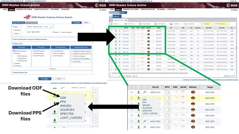
You can search for specific observation targets, regions, or sources on the main XMM Science Archive (XSA) in Europe or from the HEASARC at NASA Goddard (Xamin). These will provide you with important information about a specific observation, including the ObsID for that observation. Aside from the ObsID, the archives can provide metadata on the observations, including the duration of the observation, when the observations were taken, in which orbit XMM performed the observation, and much more.
The online search interfaces can also cover regions of the sky if you are unsure of the specific target or source. Sometimes an observation is made of a target close by and covers the target or source you are actually looking for.
Data can be downloaded from both the main XMM Science Archive (XSA) in Europe or from the HEASARC at NASA Goddard (Xamin). Below we show the interface for the XSA. After that we show the Xamin web interface. In both examples we show a search for the galaxy NGC 3079.
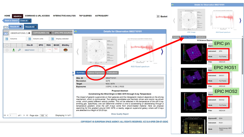
If you click on a single ObsID it will display more information. You can view basic images and see what instruments were used and what mode they were in.
Data from recent (< 1 year) observations are proprietary and to download the data from the XSA you will need to log in using a username and password. Proprietary data from the HEASARC can be downloaded but will be encrypted. You will need an encryption key to work with the data. Data older than 1 year is open and free to use. If you, or someone you are working with, has been awarded observation time on XMM you will receive instructions on how to access your proprietary data.
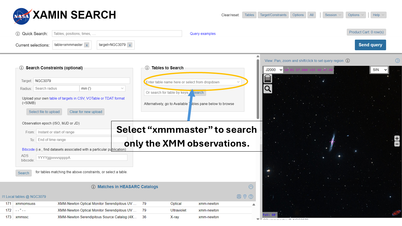
The Xamin web interface contains much more than just XMM data. It also contains data from the Chandra X-ray telescope, and other x-ray and gamma ray telescopes. It also has collections of survey data from infrared, optical, and UV telescopes. To search only XMM data you will need to select “xmmmaster” from the list of “Tables to Search”.
Data Analysis
X-ray data analysis deals primarily with running code to filter the event lists to pull the few photons you want out of the noise from the ambient background and the instruments. X-ray data is filtered and analyzed using specially written software.
XMM uses an analysis software package called the Science Analysis System (SAS). SAS was written specifically for XMM, but it is possible to use similar software written for other x-ray telescopes on XMM data. Individual functions, or pieces of SAS code are called tasks. Each ‘SAS task’ can be run from the command line on Linux or Mac computers or using the Windows Subsystem for Linux (WSL2) or a SAS Docker image or Virtual Machine. Alternatively, there is a GUI which comes with SAS that you can use to run SAS tasks.
SAS can be installed on your individual computer (you may want to have someone familiar with SAS to help you). To use SAS, you will need to install all dependencies, including HEASoft, and a few other Linux/Mac packages.
Instructions for installing SAS on Linux, Mac, WSL2, Docker, or a Virtual Machine are found at the link below.
If you have SAS installed on your own machine you should have downloaded a large amount of calibration data (>7 GB). SAS tasks used for calibration (cfibuild and odfingest) will access the calibration data for you and create the files you need for your particular data. Unless you get deep into the weeds of x-ray data analysis you will never actually need to look at the calibration data.
There is a Python wrapper for SAS called pySAS. pySAS is installed
separately from SAS using the command pip install xmmpysas. pySAS has a
few extra Python functions for dealing with XMM data, but mostly it provides a
way of calling SAS tasks from a Python environment. It is also designed to be
used with an online science platform such as Fornax, SciServer, or DataLabs.
X-ray Images
The EPIC cameras (MOS1, MOS2, pn) in imaging mode can make x-ray images. Unfiltered x-ray images almost always contain a lot of noise, as seen below. Below you can see the seven detectors that make up the MOS 1 camera. The large round circle across all the detectors is the aperture of the telescope. You just hope that what you are trying to observe doesn’t fall on any of the gaps between the chips!
There is a lot of radiation in space, from solar flares to radiation from the Van Allen Belt around the earth, and all of that must be filtered out. Some careful filtering will produce a better image like that shown below, though there still is plenty of background radiation from the rest of the universe.
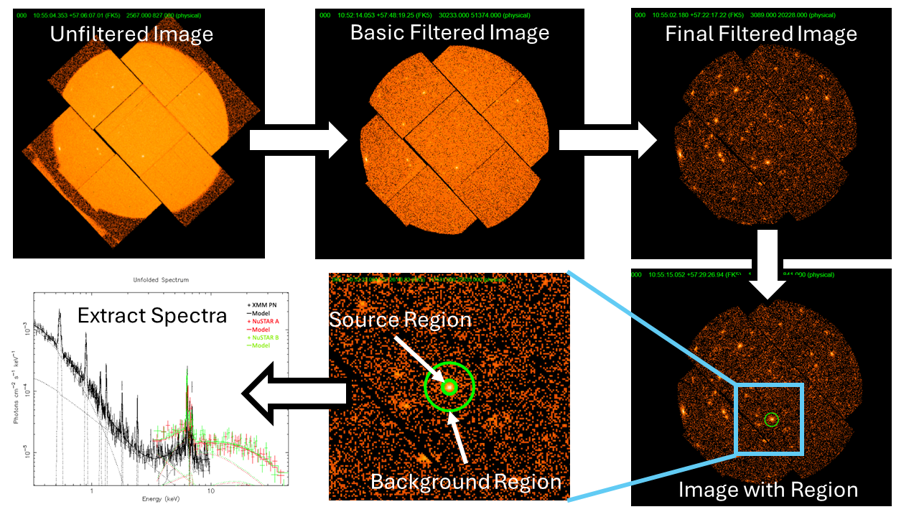
After filtering you will usually want to select a single source and extract the spectra. Above shows the selection of a single region around a single source. Then we show the same source, zoomed in, with a source region and a surrounding background region.
The background region will be used to calibrate the spectrum from the source. The selection of regions can be done using the standard program ds9. You will use SAS tasks to extract the source and background spectra. The spectra can then be fit using something like XSPEC which is part of HEASoft.
The Reality of X-Ray Spectra
In reality most x-ray spectra do not look very nice. In fact, a lot of x-ray spectra look downright horrible. For example,
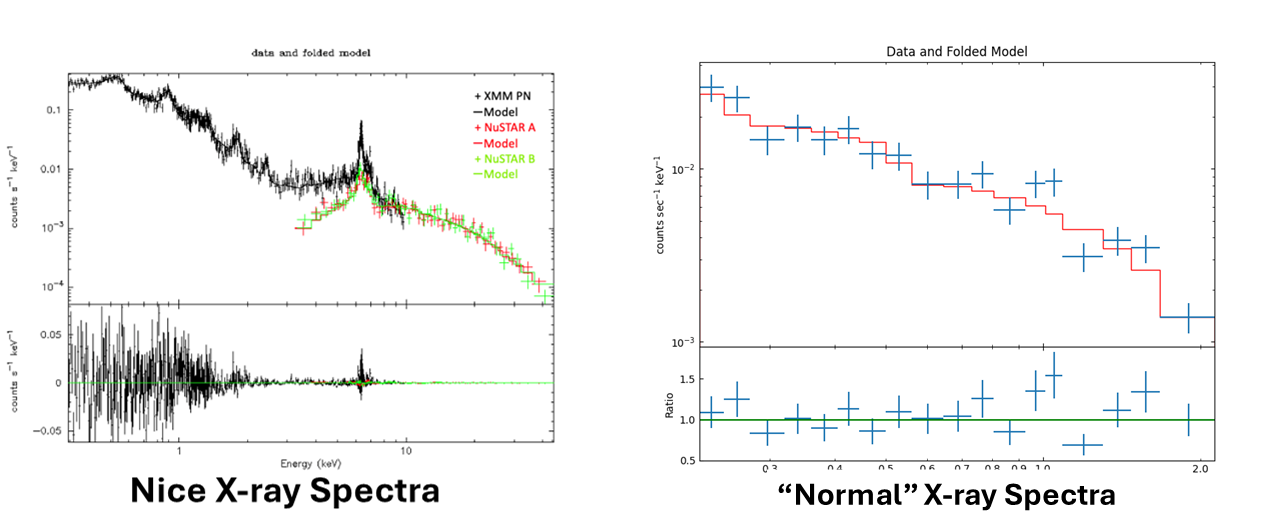
On the left we have a nice x-ray spectrum with interesting features. On the right we have what a “normal” x-ray spectra looks like. Don’t be shocked if you extract the spectra from a source and it doesn’t look like anything. Sometimes you need to perform careful filtering followed by careful modeling using XSPEC in order to get something resembling a typical light spectrum.
The spectrum on the left was carefully prepared from a bright x-ray source with a large number of photons in the event list. The spectrum on the right was from a much dimmer source with only basic filtering. At the higher end of the spectrum there is a large amount of uncertainty. The size of the bins had to be increased significantly to make the error bars reasonable. Getting something useful will take some time and experience.
The spectra shown above all come from one of the three EPIC cameras. On the left the spectrum is from the pn camera. On the right it is from the MOS1 camera. Both cameras were in imaging mode. Better x-ray spectra can be made using the RGS cameras on XMM. We will explain RGS spectra down below. The RGS cameras cannot make images like the EPIC cameras can.
Timing Mode
The second major mode for the EPIC cameras is timing mode. Timing mode deals with how an x-ray source, and its spectra, changes over time, sometimes on a very short time scale. In imaging mode, the “time resolution” of the MOS cameras is 2.6 seconds. In timing mode, the time resolution is 1.75 milliseconds (ms). For the pn, imaging mode has a time resolution of 73.4 ms, but for timing mode, it has a time resolution of 0.03 ms (or 30 µs). The pn has a mode called burst mode that has a resolution of 7 µs.
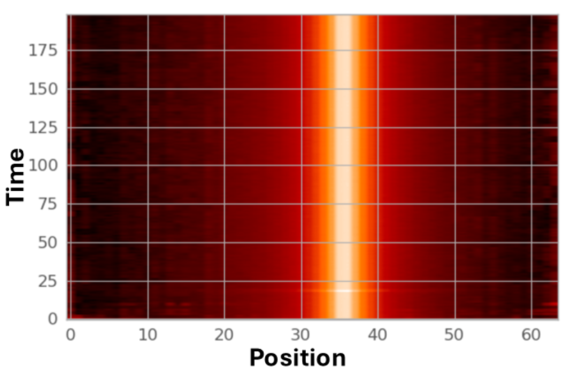
A basic diagnostic image of timing mode data is shown below. The x-axis has position data, while the y-axis has time data. The targeted x-ray source is the bright stripe between pixels #30 and #40. The idea is to extract the events generated by the bright x-ray source and then analyze the data using a purpose-built analysis code such as Xronos, which is part of HEASoft.
Depending on their area of research, some observers may never use timing mode, while others may exclusively use timing mode. Your advisor/mentor can explain things further depending on what you are observing and what the focus of the research is.
RGS Spectra
You would hope that all spectra produced by the RGS look like the ones shown below, but the reality is that like the spectra made using the MOS cameras, most RGS spectra don’t look as nice as the ones shown below. Additionally, it takes some experience, time, and effort to produce RGS spectra like those shown below. Modeling, fitting, and interpreting the data also takes experience, time, and effort.
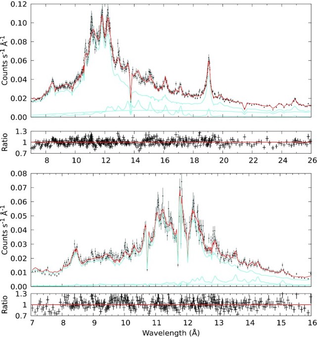
Image from Gatuzz et al. MNRAS, 2021. https://doi.org/10.1093/mnras/stab2661
Glossary of Terms
- SAS
Science Analysis Software, the basic code used to analyze XMM data.
- SAS Tasks
A task is a single stand-alone function, or piece of code, in SAS.
- pySAS
Python wrapper for SAS.
- EPIC Cameras
The three imaging x-ray cameras on XMM. They consist of,
MOS 1 (also known as EMOS1)
MOS 2 (also known as EMOS2)
pn (by convention the pn is lowercase, except when it is called EPN)
- RGS
The Reflection Grating Spectrometer, high resolution spectrometer on XMM.
- OM
Optical Monitor, an optical/UV telescope on XMM.
- Event List
A file containing a list of all high energy photons to strike the detector. The basic source of x-ray data.
- Obs ID
Observation ID, a unique 10-digit number assigned to each observation.
- ODF
Observation Data Files, raw data files.
- PPS
Processing Pipeline Subsystem files. PPS files include event lists, source lists, multi-band images, background-subtracted spectra, and light curves for sufficiently bright individual sources. The user has the option to download PPS data files instead of, or in addition to, the raw ODF files.
- The Pipeline
A standard set of SAS tasks run on all ODFs. Produces PPS files.
- XSA
XMM-Newton Science Archive: XMM data archive maintained by ESA.
- Xamin
NASA’s equivalent of the XSA (but contains more than just XMM data).
- HEASARC
The High Energy Astrophysics Science Archive Research Center (HEASARC) at NASA. Maintains an archive of all data from x-ray and gamma ray space telescopes affiliated with NASA, including XMM.
- HEASoft
High Energy Analysis Software (HEASoft), analysis code written for x-ray and gamma ray telescopes. SAS depends on HEASoft, and HEASoft must be installed and initialized before SAS can be used. HEASoft is maintained by the HEASARC.
- Imaging Mode
Used by the three EPIC cameras to produce x-ray images. You can extract spectra from individual regions in the image.
- Timing Mode
Used by the three EPIC cameras to produce x-ray timing data.
- Fornax
Online science platform where you can do XMM data analysis. Developed and maintained by NASA.
- SciServer
Online science platform where you can do XMM data analysis. Affiliated with NASA. Maintained by Johns Hopkins University.
- Datalabs
Online science platform where you can do XMM data analysis. Developed and maintained by ESA.
Links Used in this Guide
Where to get Help
Email the NASA XMM help desk directly at: - xmmhelp@athena.gsfc.nasa.gov
NASA HEASARC (including XMM) helpdesk web portal: - https://heasarc.gsfc.nasa.gov/cgi-bin/Feedback
Email the ESA XMM help desk directly at: - xmmhelp@sciops.esa.int
ESA XMM helpdesk web portal: - https://www.cosmos.esa.int/web/xmm-newton/xmm-newton-helpdesk
Document last updated: 2026-07-15